# Backpropagation {#sec-backpropagation}
## Motivace: Jak trénovat hluboké sítě?
Máme neuronovou síť s miliony parametrů. Jak spočítáme gradient loss funkce podle každého z nich? Ruční derivování by trvalo roky. Numerická aproximace by byla pomalá a nepřesná.
Řešením je **backpropagation** (zpětné šíření chyby) - elegantní algoritmus, který využívá **řetízkové pravidlo** k efektivnímu výpočtu všech gradientů v jednom průchodu sítí.
```{python}
import numpy as np
import matplotlib.pyplot as plt
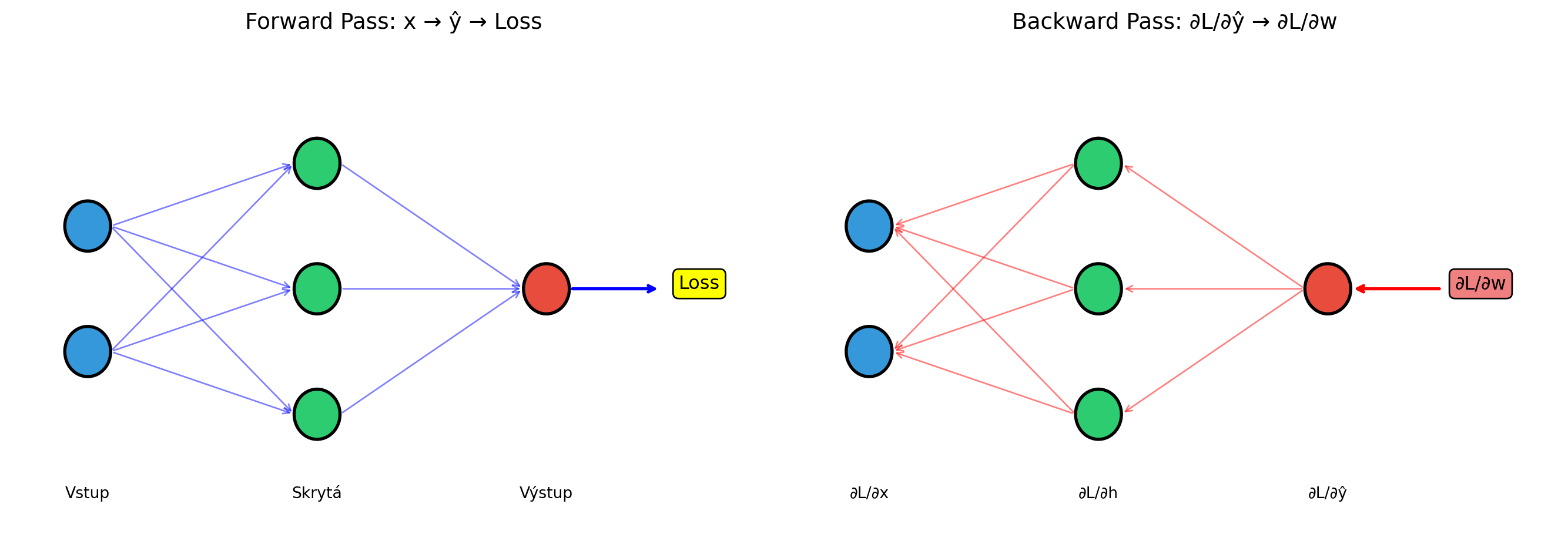
# Vizualizace forward a backward pass
fig, (ax1, ax2) = plt.subplots(1, 2, figsize=(14, 5))
# Forward pass
ax1.set_xlim(0, 10)
ax1.set_ylim(0, 6)
# Vrstvy
layers_x = [1, 4, 7]
layers_n = [2, 3, 1]
for l, (x, n) in enumerate(zip(layers_x, layers_n)):
for i in range(n):
y = 3 + (i - (n-1)/2) * 1.5
color = '#3498db' if l == 0 else '#2ecc71' if l == 1 else '#e74c3c'
circle = plt.Circle((x, y), 0.3, color=color, ec='black', lw=2)
ax1.add_patch(circle)
# Šipky forward
for i in range(2):
y1 = 3 + (i - 0.5) * 1.5
for j in range(3):
y2 = 3 + (j - 1) * 1.5
ax1.annotate('', xy=(3.7, y2), xytext=(1.3, y1),
arrowprops=dict(arrowstyle='->', color='blue', alpha=0.5))
for j in range(3):
y1 = 3 + (j - 1) * 1.5
ax1.annotate('', xy=(6.7, 3), xytext=(4.3, y1),
arrowprops=dict(arrowstyle='->', color='blue', alpha=0.5))
# Loss
ax1.annotate('Loss', xy=(9, 3), fontsize=12, ha='center',
bbox=dict(boxstyle='round', facecolor='yellow', edgecolor='black'))
ax1.annotate('', xy=(8.5, 3), xytext=(7.3, 3),
arrowprops=dict(arrowstyle='->', color='blue', lw=2))
ax1.set_title('Forward Pass: x → ŷ → Loss', fontsize=14)
ax1.text(1, 0.5, 'Vstup', ha='center')
ax1.text(4, 0.5, 'Skrytá', ha='center')
ax1.text(7, 0.5, 'Výstup', ha='center')
ax1.axis('off')
# Backward pass
ax2.set_xlim(0, 10)
ax2.set_ylim(0, 6)
for l, (x, n) in enumerate(zip(layers_x, layers_n)):
for i in range(n):
y = 3 + (i - (n-1)/2) * 1.5
color = '#3498db' if l == 0 else '#2ecc71' if l == 1 else '#e74c3c'
circle = plt.Circle((x, y), 0.3, color=color, ec='black', lw=2)
ax2.add_patch(circle)
# Šipky backward (opačný směr, červené)
for i in range(2):
y1 = 3 + (i - 0.5) * 1.5
for j in range(3):
y2 = 3 + (j - 1) * 1.5
ax2.annotate('', xy=(1.3, y1), xytext=(3.7, y2),
arrowprops=dict(arrowstyle='->', color='red', alpha=0.5))
for j in range(3):
y1 = 3 + (j - 1) * 1.5
ax2.annotate('', xy=(4.3, y1), xytext=(6.7, 3),
arrowprops=dict(arrowstyle='->', color='red', alpha=0.5))
ax2.annotate('∂L/∂w', xy=(9, 3), fontsize=12, ha='center',
bbox=dict(boxstyle='round', facecolor='lightcoral', edgecolor='black'))
ax2.annotate('', xy=(7.3, 3), xytext=(8.5, 3),
arrowprops=dict(arrowstyle='->', color='red', lw=2))
ax2.set_title('Backward Pass: ∂L/∂ŷ → ∂L/∂w', fontsize=14)
ax2.text(1, 0.5, '∂L/∂x', ha='center')
ax2.text(4, 0.5, '∂L/∂h', ha='center')
ax2.text(7, 0.5, '∂L/∂ŷ', ha='center')
ax2.axis('off')
plt.tight_layout()
plt.show()
```
## Řetízkové pravidlo v akcí
Připomeňme si řetízkové pravidlo z kapitoly o derivacích:
::: {.callout-note}
## Řetízkové pravidlo
Pokud $y = f(g(x))$, pak:
$$\frac{dy}{dx} = \frac{dy}{dg} \cdot \frac{dg}{dx}$$
Pro složitější kompozice:
$$\frac{d}{dx}[f(g(h(x)))] = f'(g(h(x))) \cdot g'(h(x)) \cdot h'(x)$$
:::
Neuronová síť je právě taková složená funkce - a backpropagation aplikuje řetízkové pravidlo systematicky.
```{python}
# Jednoduchý příklad řetízkového pravidla
# y = (2x + 3)^2

def forward(x):
    a = 2 * x + 3    # První operace
    y = a ** 2       # Druhá operace
    return y, a

def backward(x, a):
    # dy/da = 2a
    dy_da = 2 * a
    # da/dx = 2
    da_dx = 2
    # dy/dx = dy/da * da/dx
    dy_dx = dy_da * da_dx
    return dy_dx

x = 2
y, a = forward(x)
grad = backward(x, a)

print("Příklad: y = (2x + 3)²")
print(f"x = {x}")
print(f"a = 2x + 3 = {a}")
print(f"y = a² = {y}")
print(f"\nBackward:")
print(f"dy/da = 2a = {2*a}")
print(f"da/dx = 2")
print(f"dy/dx = dy/da · da/dx = {grad}")
print(f"\nOvěření: y' = 2·2·(2x+3) = 4(2·{x}+3) = {4*(2*x+3)}")
```
## Backpropagation krok za krokem
Uvažujme jednoduchou síť s jednou skrytou vrstvou:
$$\hat{y} = \sigma_2(W_2 \cdot \sigma_1(W_1 \cdot x + b_1) + b_2)$$
```{python}
import numpy as np

class SimpleNetwork:
    """Jednoduchá síť s jednou skrytou vrstvou pro demonstraci backprop."""

    def __init__(self, input_size, hidden_size, output_size):
        # Inicializace vah
        np.random.seed(42)
        self.W1 = np.random.randn(hidden_size, input_size) * 0.5
        self.b1 = np.zeros(hidden_size)
        self.W2 = np.random.randn(output_size, hidden_size) * 0.5
        self.b2 = np.zeros(output_size)

        # Pro uložení mezivýsledků
        self.cache = {}

    def sigmoid(self, z):
        return 1 / (1 + np.exp(-np.clip(z, -500, 500)))

    def sigmoid_derivative(self, a):
        return a * (1 - a)

    def forward(self, x):
        """Forward pass - uložíme mezivýsledky pro backward."""
        self.cache['x'] = x

        # Vrstva 1
        self.cache['z1'] = self.W1 @ x + self.b1
        self.cache['a1'] = self.sigmoid(self.cache['z1'])

        # Vrstva 2
        self.cache['z2'] = self.W2 @ self.cache['a1'] + self.b2
        self.cache['a2'] = self.sigmoid(self.cache['z2'])

        return self.cache['a2']

    def backward(self, y_true):
        """Backward pass - spočítáme gradienty."""
        x = self.cache['x']
        a1 = self.cache['a1']
        a2 = self.cache['a2']

        # Výstupní vrstva
        # dL/da2 pro MSE loss: 2(a2 - y)
        dL_da2 = 2 * (a2 - y_true)
        # da2/dz2 = sigmoid'(z2) = a2 * (1 - a2)
        da2_dz2 = self.sigmoid_derivative(a2)
        # dL/dz2 = dL/da2 * da2/dz2
        dL_dz2 = dL_da2 * da2_dz2

        # Gradienty W2, b2
        # dL/dW2 = dL/dz2 * dz2/dW2 = dL/dz2 * a1^T
        dL_dW2 = np.outer(dL_dz2, a1)
        dL_db2 = dL_dz2

        # Skrytá vrstva
        # dL/da1 = W2^T * dL/dz2
        dL_da1 = self.W2.T @ dL_dz2
        da1_dz1 = self.sigmoid_derivative(a1)
        dL_dz1 = dL_da1 * da1_dz1

        # Gradienty W1, b1
        dL_dW1 = np.outer(dL_dz1, x)
        dL_db1 = dL_dz1

        return {
            'dW1': dL_dW1, 'db1': dL_db1,
            'dW2': dL_dW2, 'db2': dL_db2
        }

# Demonstrace
net = SimpleNetwork(2, 3, 1)
x = np.array([1.0, 0.5])
y_true = np.array([1.0])

# Forward
y_pred = net.forward(x)
print("Forward Pass:")
print(f"  Vstup x: {x}")
print(f"  z1 = W1·x + b1: {net.cache['z1']}")
print(f"  a1 = σ(z1): {net.cache['a1']}")
print(f"  z2 = W2·a1 + b2: {net.cache['z2']}")
print(f"  a2 = σ(z2): {net.cache['a2']}")
print(f"  Predikce: {y_pred[0]:.4f}")

# Backward
grads = net.backward(y_true)
print(f"\nBackward Pass:")
print(f"  dL/dW2 shape: {grads['dW2'].shape}")
print(f"  dL/dW1 shape: {grads['dW1'].shape}")
print(f"  dL/db2: {grads['db2']}")
print(f"  dL/db1: {grads['db1']}")
```
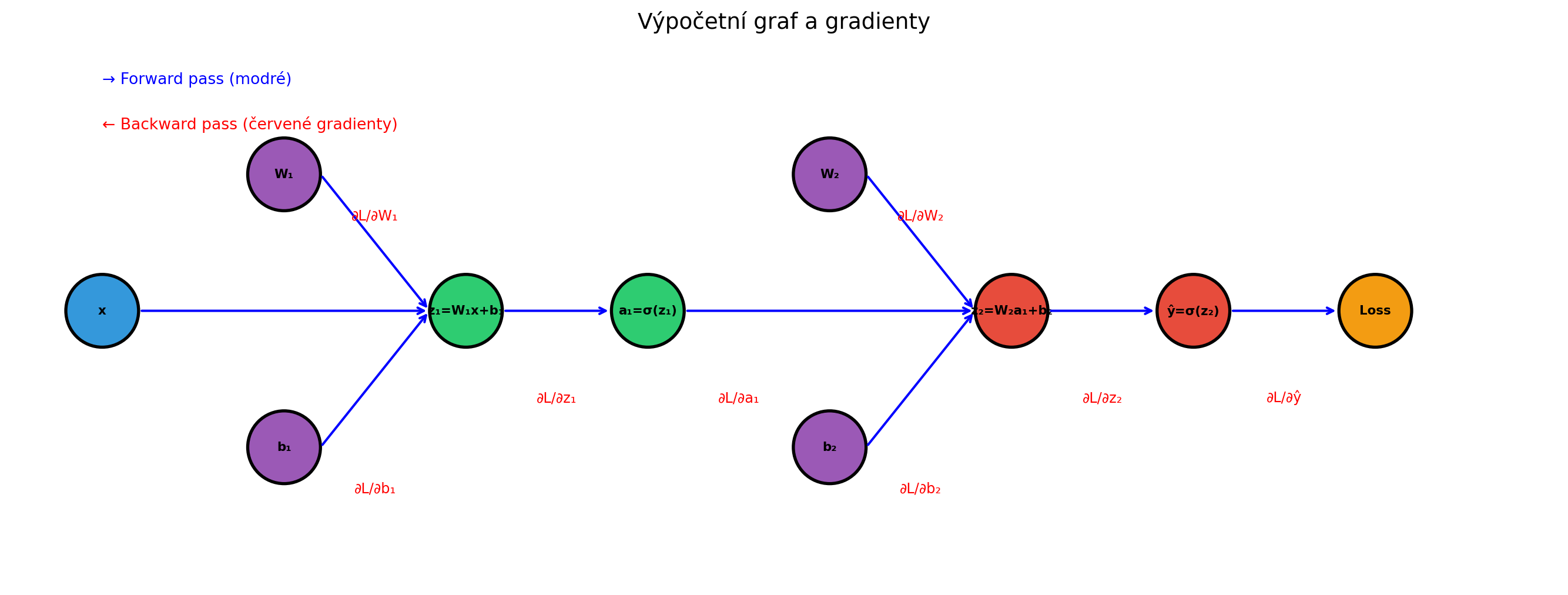
## Vizualizace výpočetního grafu
```{python}
import matplotlib.pyplot as plt

fig, ax = plt.subplots(figsize=(14, 8))

# Uzly výpočetního grafu
nodes = {
    'x': (0, 3, 'x', '#3498db'),
    'W1': (2, 4.5, 'W₁', '#9b59b6'),
    'b1': (2, 1.5, 'b₁', '#9b59b6'),
    'z1': (4, 3, 'z₁=W₁x+b₁', '#2ecc71'),
    'a1': (6, 3, 'a₁=σ(z₁)', '#2ecc71'),
    'W2': (8, 4.5, 'W₂', '#9b59b6'),
    'b2': (8, 1.5, 'b₂', '#9b59b6'),
    'z2': (10, 3, 'z₂=W₂a₁+b₂', '#e74c3c'),
    'a2': (12, 3, 'ŷ=σ(z₂)', '#e74c3c'),
    'L': (14, 3, 'Loss', '#f39c12'),
}

# Kreslení uzlů
for name, (x, y, label, color) in nodes.items():
    circle = plt.Circle((x, y), 0.4, color=color, ec='black', lw=2)
    ax.add_patch(circle)
    ax.text(x, y, label, ha='center', va='center', fontsize=8, fontweight='bold')

# Hrany (forward)
edges_forward = [
    ('x', 'z1'), ('W1', 'z1'), ('b1', 'z1'),
    ('z1', 'a1'), ('a1', 'z2'), ('W2', 'z2'), ('b2', 'z2'),
    ('z2', 'a2'), ('a2', 'L')
]

for start, end in edges_forward:
    x1, y1 = nodes[start][0], nodes[start][1]
    x2, y2 = nodes[end][0], nodes[end][1]
    ax.annotate('', xy=(x2-0.4, y2), xytext=(x1+0.4, y1),
               arrowprops=dict(arrowstyle='->', color='blue', lw=1.5))

# Popisky gradientů
grad_labels = [
    (13, 2, '∂L/∂ŷ'),
    (11, 2, '∂L/∂z₂'),
    (9, 4, '∂L/∂W₂'),
    (9, 1, '∂L/∂b₂'),
    (7, 2, '∂L/∂a₁'),
    (5, 2, '∂L/∂z₁'),
    (3, 4, '∂L/∂W₁'),
    (3, 1, '∂L/∂b₁'),
]

for x, y, label in grad_labels:
    ax.text(x, y, label, ha='center', fontsize=9, color='red')

ax.set_xlim(-1, 16)
ax.set_ylim(0, 6)
ax.set_aspect('equal')
ax.axis('off')
ax.set_title('Výpočetní graf a gradienty', fontsize=14)

# Legenda
ax.text(0, 5.5, '→ Forward pass (modré)', color='blue', fontsize=10)
ax.text(0, 5.0, '← Backward pass (červené gradienty)', color='red', fontsize=10)

plt.tight_layout()
plt.show()
```
## Odvození gradientů
Pro MSE loss $L = (ŷ - y)^2$:
```{python}
print("Odvození gradientů (MSE loss):")
print("=" * 50)
print("\n1. Výstupní vrstva:")
print("   L = (ŷ - y)²")
print("   ∂L/∂ŷ = 2(ŷ - y)")
print()
print("   ŷ = σ(z₂)")
print("   ∂ŷ/∂z₂ = σ'(z₂) = ŷ(1 - ŷ)")
print()
print("   ∂L/∂z₂ = ∂L/∂ŷ · ∂ŷ/∂z₂ = 2(ŷ - y) · ŷ(1 - ŷ)")
print()
print("   z₂ = W₂ · a₁ + b₂")
print("   ∂L/∂W₂ = ∂L/∂z₂ · a₁ᵀ")
print("   ∂L/∂b₂ = ∂L/∂z₂")
print()
print("2. Skrytá vrstva:")
print("   ∂L/∂a₁ = W₂ᵀ · ∂L/∂z₂")
print("   ∂L/∂z₁ = ∂L/∂a₁ · σ'(z₁)")
print()
print("   ∂L/∂W₁ = ∂L/∂z₁ · xᵀ")
print("   ∂L/∂b₁ = ∂L/∂z₁")
```
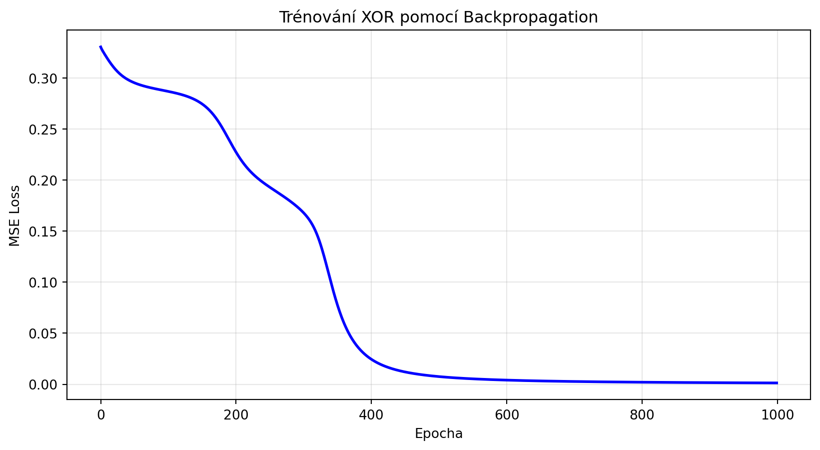
## Trénování s backpropagation
```{python}
# Kompletní trénování
import numpy as np
import matplotlib.pyplot as plt

np.random.seed(42)

# XOR data
X = np.array([[0, 0], [0, 1], [1, 0], [1, 1]])
y = np.array([[0], [1], [1], [0]])

# Síť
net = SimpleNetwork(2, 4, 1)

# Trénování
learning_rate = 1.0
losses = []

for epoch in range(1000):
    epoch_loss = 0

    for xi, yi in zip(X, y):
        # Forward
        y_pred = net.forward(xi)
        loss = (y_pred - yi) ** 2
        epoch_loss += loss[0]

        # Backward
        grads = net.backward(yi)

        # Update
        net.W2 -= learning_rate * grads['dW2']
        net.b2 -= learning_rate * grads['db2']
        net.W1 -= learning_rate * grads['dW1']
        net.b1 -= learning_rate * grads['db1']

    losses.append(epoch_loss / len(X))

    if (epoch + 1) % 200 == 0:
        print(f"Epocha {epoch+1}: Loss = {losses[-1]:.4f}")

# Výsledky
print("\nPredikce po trénování:")
for xi, yi in zip(X, y):
    pred = net.forward(xi)
    print(f"  {xi} -> {pred[0]:.4f} (target: {yi[0]})")

# Vizualizace
plt.figure(figsize=(10, 5))
plt.plot(losses, 'b-', lw=2)
plt.xlabel('Epocha')
plt.ylabel('MSE Loss')
plt.title('Trénování XOR pomocí Backpropagation')
plt.grid(True, alpha=0.3)
plt.show()
```
## Backpropagation v PyTorch
PyTorch automaticky počítá gradienty pomocí autograd:
```{python}
import torch
import torch.nn as nn

# Jednoduchá síť
class Net(nn.Module):
    def __init__(self):
        super().__init__()
        self.fc1 = nn.Linear(2, 4)
        self.fc2 = nn.Linear(4, 1)

    def forward(self, x):
        x = torch.sigmoid(self.fc1(x))
        x = torch.sigmoid(self.fc2(x))
        return x

torch.manual_seed(42)
model = Net()
criterion = nn.MSELoss()

# Data
X = torch.FloatTensor([[0, 0], [0, 1], [1, 0], [1, 1]])
y = torch.FloatTensor([[0], [1], [1], [0]])

# Forward pass
y_pred = model(X)
loss = criterion(y_pred, y)

print("Forward pass:")
print(f"  Predikce: {y_pred.detach().numpy().flatten()}")
print(f"  Loss: {loss.item():.4f}")

# Backward pass - PyTorch spočítá gradienty automaticky!
loss.backward()

print("\nBackward pass (gradienty):")
for name, param in model.named_parameters():
    print(f"  {name}: grad shape = {param.grad.shape}")
    print(f"         grad mean = {param.grad.mean().item():.4f}")
```
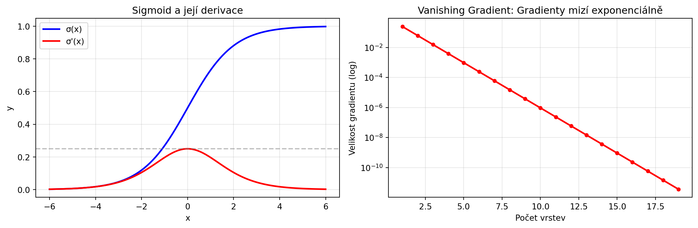
## Gradient Flow a problémy
### Vanishing Gradient
Při průchodu mnoha vrstvami se gradienty mohou "ztratit":
```{python}
# Demonstrace vanishing gradient s sigmoid
import numpy as np
import matplotlib.pyplot as plt

def sigmoid(x):
    return 1 / (1 + np.exp(-x))

def sigmoid_derivative(x):
    s = sigmoid(x)
    return s * (1 - s)

# Gradient sigmoid je maximálně 0.25
x = np.linspace(-6, 6, 100)

fig, (ax1, ax2) = plt.subplots(1, 2, figsize=(12, 4))

ax1.plot(x, sigmoid(x), 'b-', lw=2, label='σ(x)')
ax1.plot(x, sigmoid_derivative(x), 'r-', lw=2, label="σ'(x)")
ax1.axhline(y=0.25, color='gray', linestyle='--', alpha=0.5)
ax1.set_xlabel('x')
ax1.set_ylabel('y')
ax1.set_title('Sigmoid a její derivace')
ax1.legend()
ax1.grid(True, alpha=0.3)

# Gradient po průchodu n vrstvami
n_layers = np.arange(1, 20)
# V nejlepším případě každá vrstva násobí gradient 0.25
gradient_decay = 0.25 ** n_layers

ax2.semilogy(n_layers, gradient_decay, 'r.-', lw=2, markersize=8)
ax2.set_xlabel('Počet vrstev')
ax2.set_ylabel('Velikost gradientu (log)')
ax2.set_title('Vanishing Gradient: Gradienty mizí exponenciálně')
ax2.grid(True, alpha=0.3)

plt.tight_layout()
plt.show()

print("Po 10 vrstvách je gradient pouze:", 0.25**10)
```
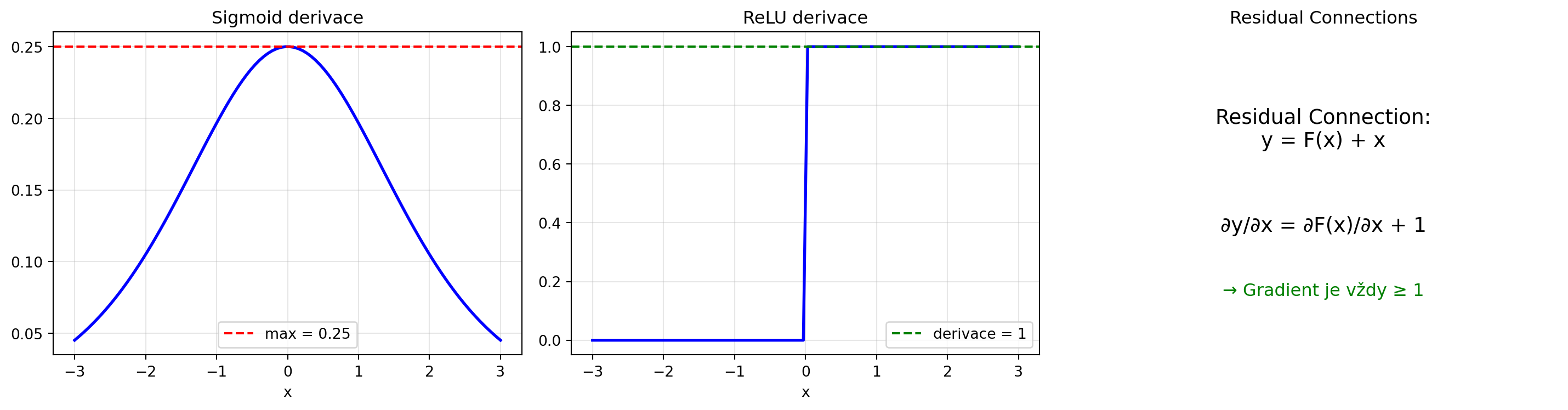
### Řešení: ReLU a Residual Connections
```{python}
# ReLU derivace
import numpy as np
import matplotlib.pyplot as plt

def relu(x):
    return np.maximum(0, x)

def relu_derivative(x):
    return (x > 0).astype(float)

x = np.linspace(-3, 3, 100)

fig, axes = plt.subplots(1, 3, figsize=(15, 4))

# Sigmoid
ax = axes[0]
ax.plot(x, sigmoid_derivative(x), 'b-', lw=2)
ax.axhline(y=0.25, color='red', linestyle='--', label='max = 0.25')
ax.set_title('Sigmoid derivace')
ax.set_xlabel('x')
ax.legend()
ax.grid(True, alpha=0.3)

# ReLU
ax = axes[1]
ax.plot(x, relu_derivative(x), 'b-', lw=2)
ax.axhline(y=1, color='green', linestyle='--', label='derivace = 1')
ax.set_title('ReLU derivace')
ax.set_xlabel('x')
ax.legend()
ax.grid(True, alpha=0.3)

# Residual connection
ax = axes[2]
ax.text(0.5, 0.7, 'Residual Connection:\ny = F(x) + x', ha='center', va='center',
        fontsize=14, transform=ax.transAxes)
ax.text(0.5, 0.4, '∂y/∂x = ∂F(x)/∂x + 1', ha='center', va='center',
        fontsize=14, transform=ax.transAxes)
ax.text(0.5, 0.2, '→ Gradient je vždy ≥ 1', ha='center', va='center',
        fontsize=12, color='green', transform=ax.transAxes)
ax.axis('off')
ax.set_title('Residual Connections')

plt.tight_layout()
plt.show()
```
## Gradient Checking
Pro ověření správnosti backpropagation můžeme porovnat s numerickým gradientem:
```{python}
import numpy as np

def numerical_gradient(f, params, eps=1e-5):
    """Numerický gradient pro ověření."""
    grads = []

    for i, p in enumerate(params):
        grad = np.zeros_like(p)

        for idx in np.ndindex(p.shape):
            old_val = p[idx]

            p[idx] = old_val + eps
            loss_plus = f()

            p[idx] = old_val - eps
            loss_minus = f()

            p[idx] = old_val

            grad[idx] = (loss_plus - loss_minus) / (2 * eps)

        grads.append(grad)

    return grads

# Test gradient checking
net = SimpleNetwork(2, 3, 1)
x = np.array([1.0, 0.5])
y_true = np.array([1.0])

# Analytický gradient (backprop)
y_pred = net.forward(x)
analytical_grads = net.backward(y_true)

# Numerický gradient
def compute_loss():
    pred = net.forward(x)
    return ((pred - y_true) ** 2).sum()

numerical_grads = numerical_gradient(compute_loss, [net.W1, net.b1, net.W2, net.b2])

# Porovnání
print("Gradient Checking:")
print("-" * 50)
for name, analytical, numerical in [
    ('dW1', analytical_grads['dW1'], numerical_grads[0]),
    ('db1', analytical_grads['db1'], numerical_grads[1]),
    ('dW2', analytical_grads['dW2'], numerical_grads[2]),
    ('db2', analytical_grads['db2'], numerical_grads[3])
]:
    diff = np.abs(analytical - numerical).max()
    status = "✓ OK" if diff < 1e-5 else "✗ CHYBA"
    print(f"{name}: max rozdíl = {diff:.2e} {status}")
```
## Řešené příklady
### Příklad 1: Ruční backprop pro malou síť
**Zadání**: Pro síť $y = \sigma(w_2 \cdot \sigma(w_1 \cdot x + b_1) + b_2)$ s $w_1=0.5$, $b_1=0.1$, $w_2=0.8$, $b_2=-0.2$, vstupem $x=1$ a cílem $y_{true}=1$ spočítejte gradienty.
**Řešení**:
```{python}
# Parametry
import numpy as np

w1, b1 = 0.5, 0.1
w2, b2 = 0.8, -0.2
x = 1.0
y_true = 1.0

print("Forward pass:")
z1 = w1 * x + b1
print(f"  z1 = w1·x + b1 = {w1}·{x} + {b1} = {z1}")

a1 = 1 / (1 + np.exp(-z1))
print(f"  a1 = σ(z1) = {a1:.4f}")

z2 = w2 * a1 + b2
print(f"  z2 = w2·a1 + b2 = {w2}·{a1:.4f} + {b2} = {z2:.4f}")

a2 = 1 / (1 + np.exp(-z2))
print(f"  a2 = σ(z2) = {a2:.4f}")

loss = (a2 - y_true) ** 2
print(f"  Loss = (a2 - y)² = ({a2:.4f} - {y_true})² = {loss:.4f}")

print("\nBackward pass:")
# ∂L/∂a2
dL_da2 = 2 * (a2 - y_true)
print(f"  ∂L/∂a2 = 2(a2 - y) = {dL_da2:.4f}")

# ∂a2/∂z2
da2_dz2 = a2 * (1 - a2)
print(f"  ∂a2/∂z2 = a2(1-a2) = {da2_dz2:.4f}")

# ∂L/∂z2
dL_dz2 = dL_da2 * da2_dz2
print(f"  ∂L/∂z2 = ∂L/∂a2 · ∂a2/∂z2 = {dL_dz2:.4f}")

# ∂L/∂w2, ∂L/∂b2
dL_dw2 = dL_dz2 * a1
dL_db2 = dL_dz2
print(f"  ∂L/∂w2 = ∂L/∂z2 · a1 = {dL_dw2:.4f}")
print(f"  ∂L/∂b2 = ∂L/∂z2 = {dL_db2:.4f}")

# Pokračování ke skryté vrstvě
dL_da1 = dL_dz2 * w2
da1_dz1 = a1 * (1 - a1)
dL_dz1 = dL_da1 * da1_dz1
dL_dw1 = dL_dz1 * x
dL_db1 = dL_dz1

print(f"\n  ∂L/∂a1 = ∂L/∂z2 · w2 = {dL_da1:.4f}")
print(f"  ∂L/∂z1 = ∂L/∂a1 · a1(1-a1) = {dL_dz1:.4f}")
print(f"  ∂L/∂w1 = ∂L/∂z1 · x = {dL_dw1:.4f}")
print(f"  ∂L/∂b1 = ∂L/∂z1 = {dL_db1:.4f}")
```
### Příklad 2: Backprop pro batch
**Zadání**: Upravte backpropagation pro práci s batch dat.
**Řešení**:
```{python}
import numpy as np

class BatchNetwork:
    """Síť s podporou batch zpracování."""

    def __init__(self, input_size, hidden_size, output_size):
        np.random.seed(42)
        self.W1 = np.random.randn(hidden_size, input_size) * 0.5
        self.b1 = np.zeros((1, hidden_size))
        self.W2 = np.random.randn(output_size, hidden_size) * 0.5
        self.b2 = np.zeros((1, output_size))

    def forward(self, X):
        # X shape: (batch_size, input_size)
        self.X = X
        self.z1 = X @ self.W1.T + self.b1
        self.a1 = 1 / (1 + np.exp(-self.z1))
        self.z2 = self.a1 @ self.W2.T + self.b2
        self.a2 = 1 / (1 + np.exp(-self.z2))
        return self.a2

    def backward(self, y_true):
        batch_size = y_true.shape[0]

        # Výstupní vrstva
        dL_da2 = 2 * (self.a2 - y_true) / batch_size  # Průměr přes batch
        da2_dz2 = self.a2 * (1 - self.a2)
        dL_dz2 = dL_da2 * da2_dz2

        dL_dW2 = dL_dz2.T @ self.a1
        dL_db2 = dL_dz2.sum(axis=0, keepdims=True)

        # Skrytá vrstva
        dL_da1 = dL_dz2 @ self.W2
        da1_dz1 = self.a1 * (1 - self.a1)
        dL_dz1 = dL_da1 * da1_dz1

        dL_dW1 = dL_dz1.T @ self.X
        dL_db1 = dL_dz1.sum(axis=0, keepdims=True)

        return {'dW1': dL_dW1, 'db1': dL_db1, 'dW2': dL_dW2, 'db2': dL_db2}

# Test s batchem
net = BatchNetwork(2, 4, 1)
X_batch = np.array([[0, 0], [0, 1], [1, 0], [1, 1]], dtype=float)
y_batch = np.array([[0], [1], [1], [0]], dtype=float)

y_pred = net.forward(X_batch)
grads = net.backward(y_batch)

print("Batch processing:")
print(f"  Vstup shape: {X_batch.shape}")
print(f"  Výstup shape: {y_pred.shape}")
print(f"  dW1 shape: {grads['dW1'].shape}")
print(f"  dW2 shape: {grads['dW2'].shape}")
```
## Cvičení
::: {.callout-note icon=false}
## Cvičení 1: Ruční backprop
Odvoďte gradienty pro síť s ReLU aktivací místo sigmoid. Jak se liší vzorce?
:::
::: {.callout-note icon=false}
## Cvičení 2: Cross-entropy
Upravte backpropagation pro cross-entropy loss místo MSE. Jaký je gradient $\frac{\partial L}{\partial z}$ pro softmax + cross-entropy?
:::
::: {.callout-note icon=false}
## Cvičení 3: Gradient checking
Implementujte gradient checking pro síť s 3 vrstvami. Ověřte správnost vaší implementace backprop.
:::
::: {.callout-note icon=false}
## Cvičení 4: Vizualizace gradientů
Vizualizujte, jak se velikost gradientů mění v jednotlivých vrstvách během tréninku. Pozorujete vanishing nebo exploding gradients?
:::
::: {.callout-note icon=false}
## Cvičení 5: Implementace v NumPy
Implementujte plně funkční MLP s backpropagation v čistém NumPy včetně:
- Více skrytých vrstev
- Různé aktivační funkce
- Mini-batch training
- L2 regularizace
:::
## Shrnutí
::: {.callout-tip}
## Co jsme se naučili
1. **Backpropagation** využívá řetízkové pravidlo k výpočtu gradientů
2. **Forward pass** počítá predikci a ukládá mezivýsledky
3. **Backward pass** propaguje gradienty od výstupu ke vstupu
4. Pro každou vrstvu: $\frac{\partial L}{\partial W} = \frac{\partial L}{\partial z} \cdot a_{prev}^T$
5. **Vanishing gradient** je problém hlubokých sítí s sigmoid
6. **ReLU** a **residual connections** pomáhají s gradient flow
7. **Gradient checking** ověřuje správnost implementace
:::
::: {.callout-important}
## Klíčové vzorce
- **Řetízkové pravidlo**: $\frac{\partial L}{\partial w} = \frac{\partial L}{\partial z} \cdot \frac{\partial z}{\partial w}$
- **Gradient přes vrstvu**: $\frac{\partial L}{\partial a^{(l-1)}} = W^{(l)T} \cdot \frac{\partial L}{\partial z^{(l)}}$
- **Gradient vah**: $\frac{\partial L}{\partial W^{(l)}} = \frac{\partial L}{\partial z^{(l)}} \cdot (a^{(l-1)})^T$
- **Sigmoid derivace**: $\sigma'(z) = \sigma(z)(1 - \sigma(z))$
- **ReLU derivace**: $\text{ReLU}'(z) = \mathbb{1}_{z > 0}$
:::
V poslední kapitole se podíváme na **transformery** - architekturu, která revolucionalizovala zpracování přirozeného jazyka a stojí za modely jako GPT a BERT.